PPAA
所谓PPAA(Post Process Antialiasing),也叫FBAA(Filter-Based Antialiasing),是基于后处理的各种抗锯齿技术的统称。在PPAA之前,主流AA技术是MSAA(MultiSamples AA)、SSAA(SuperSamples AA)。SSAA是AA中最暴力也是最完美的解决方案,而MSAA是与硬件紧密结合的built-in AA。对于forward rendering来说,MSAA几乎是唯一的选择。
然而,MSAA这种古老的、built-in的技术,已经不太能满足现代渲染器的需求了。它有两大问题,一是MSAA会有多余的AA计算,二是MSAA不适用于deferred rendering。
鉴于MSAA的不足,PPAA就蓬勃发展起来了。PPAA强大之处在于可以自定义、且硬件无关、兼容forward/defer,所以基于PPAA的算法非常多。而其中的翘楚,SMAA(Subpixel Morphological Antialiasing),性能以及AA质量都很不错。本文将着重介绍SMAA。
值得一提的是,SMAA的前身是Jimenez's MLAA,也是同一个团队做出来的,SMAA可以认为是在质量和性能两方面都超越Jimenez's MLAA的一个进化版。所以可以先阅读Jimenez's MLAA的论文再来学习SMAA。
SMAA
SMAA的模式处理较之MLAA有了新的改进。MLAA的方法,对sharp物体的轮廓的"边角"和"锯齿角"并不能区分,导致边角也被当作锯齿角处理,导致边角被修成了圆角。而SMAA中,做了进一步的观察:对于锯齿角,大小不超过一个像素,而sharp的边角很大几率超过1个像素。因此,SMAA判断锯齿角需要计算2个像素长度的范围,也从而识别出真的边角。但也就使得SMAA的算法极为复杂。
SMAA总共3个pass:
- Pass 1,算edgeTex
- Pass 2,用edgeTex算weightTex
- Pass 3,用weightTex混合原始图像,得到抗锯齿图像
边缘纹理的计算 Edge Detection (edgeTex) (Pass 1)
锯齿问题体现在图像上几何物体的边缘处,也就是说,如果能准确地post process出图像上哪些地方是边,哪些地方不是。检测过少,锯齿边就会残留;检测过多,图像就会糊。为来更好地提升AA质量,SMAA边缘检测算法的选取非常关键。
相比基于normal map、depth map,基于颜色的边缘检测尤佳。一是因为,颜色信息容易获得,而深度图/法线图相对难获得,例如对于图像处理领取,用户提供的只有照片而已;二是因为它还有一个优点:对于做了shading后才产生的锯齿,也一样能处理(例如有梯度的toon shading)。
SMAA首推的是基于Luma(亮度)的边缘检测算法。
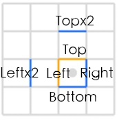
1,vertex shader,根据纹理坐标输出3组offset,每组2个边,总共6个边要检测:
    vec4 SMAA_RT_METRICS = vec4(1.0 / imgSize.x, 1.0 / imgSize.y, imgSize.x, imgSize.y);
    Offsets[0] = fma(SMAA_RT_METRICS.xyxy, vec4(-1.0, 0.0, 0.0, -1.0), texCoord.xyxy); // Left / Top Edge
    Offsets[1] = fma(SMAA_RT_METRICS.xyxy, vec4( 1.0, 0.0, 0.0,  1.0), texCoord.xyxy); // Right / Bottom Edge
    Offsets[2] = fma(SMAA_RT_METRICS.xyxy, vec4(-2.0, 0.0, 0.0, -2.0), texCoord.xyxy); // Leftx2 / Topx2 Edge
2,fragment shader,先求出当前fragment的luma值:
    // Calculate lumas:
    float3 weights = float3(0.2126, 0.7152, 0.0722);
    float L = dot(texture(colorTex, texcoord).rgb, weights);
(RGB->luma的公式来自wiki https://en.wikipedia.org/wiki/Relative_luminance )
3,算Left和Top的luma值,以及算Left和L的差值delta.x、Top和L的差值delta.y;如果delta.x < threshold.x,edges.x就等于0.0,代表不是边(因为差值很小,即亮度差异小),y方向同理:
    float Lleft = dot(texture(colorTex, offsets[0].xy).rgb, weights);
    float Ltop  = dot(texture(colorTex, offsets[0].zw).rgb, weights);

    float4 delta;
    delta.xy = abs(L - float2(Lleft, Ltop));
    float2 edges = step(threshold, delta.xy);

    if (dot(edges, float2(1.0, 1.0)) == 0.0)
        discard; // 如果2个方向都没有边,就可以排除这个fragment了
- 如果Left或Top至少有一个是边,就再进一步做检测。
    // 计算Right Bottom的luma差值
    float Lright = dot(texture(colorTex, offsets[1].xy).rgb, weights);
    float Lbottom  = dot(texture(colorTex, offsets[1].zw).rgb, weights);
    delta.zw = abs(L - float2(Lright, Lbottom)); // 和算delta.xy过程差不多

    // 分别算出x、y方向的最大luma差值
    float2 maxDelta = max(delta.xy, delta.zw);

    // 算出 Left x2 and Top x2 的luma:
    float Lleftleft = dot(texture(colorTex, offsets[2].xy).rgb, weights);
    float Ltoptop = dot(texture(colorTex, offsets[2].zw).rgb, weights);
    // 算出Left和Left x2的luma差值、Top和Top x2的luma差值
    delta.zw = abs(float2(Lleft, Ltop) - float2(Lleftleft, Ltoptop));

    // Calculate the final maximum delta:
    // x、y方向分别最终的最大luma差值
    maxDelta = max(maxDelta.xy, delta.zw);
    // x、y两个方向中取其中最大的luma差值
    float finalDelta = max(maxDelta.x, maxDelta.y);

    // Local contrast adaptation:
    float SMAA_LOCAL_CONTRAST_ADAPTATION_FACTOR = 2.0;
    // Left、Top亮度差值*2后需超过finalDelta才真的是边
    edges.xy *= step(finalDelta, SMAA_LOCAL_CONTRAST_ADAPTATION_FACTOR * delta.xy);

    return edges;
权重纹理的计算 Blending Weight Calculation (weightTex)(Pass 2)
最复杂的一个pass,需要分成多个部分讲解。
预生成searchTex
根据当前像素坐标,搜索当前这个像素对应的边的2个端点,求出2个距离值\(d_{1}、d_{2}\),是实现模式分类的关键。
因为edgeTex已经包含了边的信息,如果直接暴力搜索端点,就需要对edgeTex做非常多次的纹理采样(我没搞错的话,次数应该等于\(d_{1} + d_{2}\) )。在Jimenez's MLAA中,使用一个叫bilinear filtering的搜索技巧,能大约减少一半的纹理采样数。原理大致如下:
假设有2个要采样的相邻像素点,现在目标是用一次采样得到这2个点的'边'值:\(b_{1}、b_{2}\) (要么等于0要么等于1,代表有无边)。首先得把这个edgeTex纹理的过滤设置,设置成GL_LINEAR。这样就可以利用GPU的插值机制,通过求2个像素点连线上的某一个中间点x的纹理坐标,做一次采样,得到一个[0,1]之间的值。有了这个值后,是能够恢复出\(b_{1}、b_{2}\) 的值的。是不是很神奇?数学原理是这样的:
\[ f_{x}(b_{1},b_{2},x) = x\cdot b_{1} + (1 - x)\cdot b_{2},b_{1} = 0/1,b_{2} = 0/1 \]
(值得一提的是,在shader里需要把 \( x\cdot b_{1} + (1 - x)\cdot b_{2} \)变换成 \( x\cdot (b_{1} - b_{2} ) + b_{2} \),即lerp形式,这样可以减少一次乘法运算)
假设我们先取x=0.5,那么f的取值范围为[0, 0.5, 1],具体的映射关系为:
\( b_{1}\ \ \ b_{2}\ \ \ —— \ \ \ f \)
\( 0\ \ \ \ \ 0\ \ \ \ —— \ \ \ 0 \)
\( 0\ \ \ \ \ 1\ \ \ \ —— \ \ \ 0.5 \)
\( 1\ \ \ \ \ 0\ \ \ \ —— \ \ \ 0.5 \)
\( 1\ \ \ \ \ 1\ \ \ \ —— \ \ \ 1 \)
可以看到左右两边并不是一一对应的关系,0.5对应了2种情况。那么假设我们再取别的值,且满足\(x \neq 0.5,x \neq 0 ,x \neq 1 \),那么有:
\( b_{1}\ \ \ b_{2}\ \ \ —— \ \ \ f \)
\( 0\ \ \ \ \ 0\ \ \ \ —— \ \ \ 0 \)
\( 0\ \ \ \ \ 1\ \ \ \ —— \ \ \ 1 - x \)
\( 1\ \ \ \ \ 0\ \ \ \ —— \ \ \ x \)
\( 1\ \ \ \ \ 1\ \ \ \ —— \ \ \ 1 \)
神奇的事情发生了,左右两边满足了一一对应关系!也就是说,只需要知道x的值,就能'解码'出\(b_{1}、b_{2}\)的值!
这个bilinear filtering虽好,但它只能搜索一个方向(一维)。而在SMAA中,因为需要进一步做好模式分类,需要支持二维的edgeTex搜索。所以SMAA拓展了bilinear filtering到了二维:
\[ f_{xy}(b_{1},b_{2},b_{3},b_{4},x,y) = f_{x}(b_{1},b_{2},x) \cdot y + f_{x}(b_{3},b_{4},x) \cdot (1 - y) \]
这里增加了一个y,y和x是类似的,需要赋予一个不等于0.5的值,但需要附加一个限制是y = 0.5x(可以假设y!=0.5x去推导上面的公式,会得到无法一一对应的情况)。这样拓展后,就可以用2个常量值x、y,对\(b_{1}、b_{2}、b_{3}、b_{4}\)所有组合编码出\(2^{4} \)共16种取值情况。也就是依然可以用一个f值,反向找出\(b_{1}、b_{2}、b_{3}、b_{4}\)!
这个映射关系可以打表到代码里减少shader计算,但这样还不够,SMAA做啦进一步的优化,减少了对这个映射表的访问。作者写了一个脚本来生成一个叫searchTex的东西。先讲一下生成步骤再说用法。
首先,确定了刚才提到的常量x,y的值,x等于0.25,y等于0.5x=0.125。然后枚举16种情况,调用bilinear函数,生成映射表:
# Interpolates between two values:
def lerp(v0, v1, p):
    return v0 + (v1 - v0) * p

# Calculates the bilinear fetch for a certain edge combination:
def bilinear(e):
    # e[0]       e[1]
    #
    #          x <-------- Sample position:    (-0.25,-0.125)
    # e[2]       e[3] <--- Current pixel [3]:  (  0.0, 0.0  )
    a = lerp(e[0], e[1], 1.0 - 0.25)
    b = lerp(e[2], e[3], 1.0 - 0.25)
    return lerp(a, b, 1.0 - 0.125)

# This dict returns which edges are active for a certain bilinear fetch:
# (it's the reverse lookup of the bilinear function)
edge = {
    bilinear([0, 0, 0, 0]): [0, 0, 0, 0], # 0.0
    bilinear([0, 0, 0, 1]): [0, 0, 0, 1], # 0.65625
    bilinear([0, 0, 1, 0]): [0, 0, 1, 0], # 0.21875
    bilinear([0, 0, 1, 1]): [0, 0, 1, 1], # 0.875

    bilinear([0, 1, 0, 0]): [0, 1, 0, 0], # 0.09375
    bilinear([0, 1, 0, 1]): [0, 1, 0, 1], # 0.75
    bilinear([0, 1, 1, 0]): [0, 1, 1, 0], # 0.3125
    bilinear([0, 1, 1, 1]): [0, 1, 1, 1], # 0.96875

    bilinear([1, 0, 0, 0]): [1, 0, 0, 0], # 0.03125
    bilinear([1, 0, 0, 1]): [1, 0, 0, 1], # 0.6875
    bilinear([1, 0, 1, 0]): [1, 0, 1, 0], # 0.25
    bilinear([1, 0, 1, 1]): [1, 0, 1, 1], # 0.90625

    bilinear([1, 1, 0, 0]): [1, 1, 0, 0], # 0.125
    bilinear([1, 1, 0, 1]): [1, 1, 0, 1], # 0.78125
    bilinear([1, 1, 1, 0]): [1, 1, 1, 0], # 0.34375
    bilinear([1, 1, 1, 1]): [1, 1, 1, 1], # 1.0
}
然后观察16个bilinear值,发现它们有最大公约数0.03125,于是,可以设计一个大小为33 x 33的数组(这是因为33 = 1 / 0.03125 + 1),又因为搜索的是line,需要分左右(也只有左右2个方向),所以数组要乘2,变成66 x 33。
然后开始枚举所有pattern:
# Calculate delta distances to the left:
image = Image.new("RGB", (66, 33))
for x in range(33):
    for y in range(33):
        texcoord = 0.03125 * x, 0.03125 * y
        if texcoord[0] in edge and texcoord[1] in edge:
            edges = edge[texcoord[0]], edge[texcoord[1]]
            val = 127 * deltaLeft(*edges) # Maximize dynamic range to help compression
            image.putpixel((x, y), (val, val, val))
            #debug("left: ", texcoord, val, *edges)

# Calculate delta distances to the right:
for x in range(33):
    for y in range(33):
        texcoord = 0.03125 * x, 0.03125 * y
        if texcoord[0] in edge and texcoord[1] in edge:
            edges = edge[texcoord[0]], edge[texcoord[1]]
            val = 127 * deltaRight(*edges) # Maximize dynamic range to help compression
            image.putpixel((33 + x, y), (val, val, val))
            #debug("right: ", texcoord, val, *edges)
其中的if texcoord[0] in edge and texcoord[1] in edge意思是当前这2个纹理坐标x y,都刚好是一个f,f就对应了某四个bool值,2个f就组成一个pattern。edges = edge[texcoord[0]], edge[texcoord[1]],分别解码出了x y方向的4个bool值。接着是另外两个函数:
# Delta distance to add in the last step of searches to the left:
def deltaLeft(left, top):
    d = 0
    # If there is an edge, continue:
    if top[3] == 1:
        d += 1
    # If we previously found an edge, there is another edge and no crossing
    # edges, continue:
    if d == 1 and top[2] == 1 and left[1] != 1 and left[3] != 1:
        d += 1
    return d
# Delta distance to add in the last step of searches to the right:
def deltaRight(left, top):
    d = 0
    # If there is an edge, and no crossing edges, continue:
    if top[3] == 1 and left[1] != 1 and left[3] != 1:
        d += 1
    # If we previously found an edge, there is another edge and no crossing
    # edges, continue:
    if d == 1 and top[2] == 1 and left[0] != 1 and left[2] != 1:
        d += 1
    return d
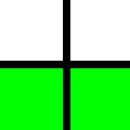
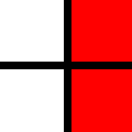
deltaLeft,就是根据x y方向2组bool值,算出一个长度补充值d,d的取值范围是0/1/2。top[3]是指当前像素在y方向上的bool值,如果为0,就是没边,d = 0;如果为1,就是有边,那么d = 1;再如果top[2]也有边,且x方向没有边(没有交叉边),那么d = 2。deltaRight过程类似。
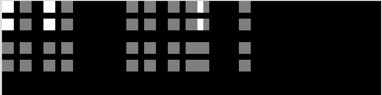
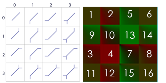
以下图为例,上面的是top,下面的是left,标绿色/红色的是边,那么经过deltaLeft运算后,下面的pattern会得到d=1(有交叉边)。
求出d后, val = 127 * d,把d映射到0/127/254,然后就可以填入到searchTex了,相当于是在生成一张三值的灰度值。
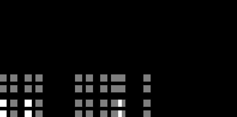
观察searchTex发现,这图有很大部分是全黑的。略显多余,于是作者补充了一个裁剪操作:
image = image.crop([0, 17, 64, 33])
image = image.transpose(Image.FLIP_TOP_BOTTOM)
把上面的17行黑色区域都裁掉,searchTex就变成了64x16的大小,符合2的幂次方,更迷你更优雅。第二行代码做了个上下翻转,用意不明。最终的searchTex如下:
searchTex会用在横向和纵向的搜索中。
预生成areaTex
areaTex是用来快速算出面积比,即混合权重的。AreaTex的生成步骤比searchTex更复杂,作者更是用了多线程来做。为了破解areaTex的魔法原理,需要慢慢剖析AreaTex.py。尽管AreaTex.py已经有不少注释,但还是很难理解。
先来看areaTex长啥样:
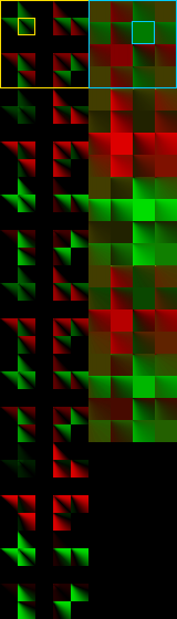
它分左右两列,左边一列七个大格(黄色框代表第一个大格),每个大格包含16个pattern的area纹理,右边一列类似,但只有五个大格(蓝色框)。有意思的是黄框大格是有镂空的,理应可以放5*5=25个小格,但只放了16个,所以有个十字架的黑色区域(原因和binear filtering有关)。因为areaTex有4个维度: ortho还是diag、哪一个大格、哪一个小格、纹理坐标,所以areaTex是一个4D的纹理。
标记下16个pattern在大格里的位置:
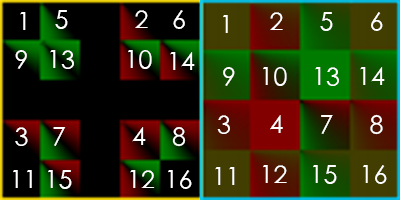
(值得一提的是,对于SMAA 1x,只会用到第一排这2个大格。)
对于orhto、并且只用SMAA 1x的情况,查询areaTex需要这么些参数:当前像素点的edge line的left方向和right方向末尾的边值e1、e2以及长度值d1、d2。e1、e2用来定位大格中的小格,d1、d2用来定位小格里的像素点。
注意,因为areaTex分辨率有限,并且需要用长度值去索引,所以对于超长的锯齿边,就行不通了。作者也加了一个#define SMAA_MAX_SEARCH_STEPS 32。32就是小格的边长的一半,因为做了一个sqrt的压缩。
areaTex的使用地方极少,只有在pass2调用了两次SMAAArea。所以关键的地方是areaTex的原理和生成(AreaTex.py)、以及SMAAArea需要的参数的计算。
areaTex的生成是brute force的,遍历每一个subsample offset、每一个pattern、每一个left distance、每一个right distance,然后算出left、right方向4个面积存到weightTex,就可以给pass 3用了。
先看如何生成Ortho(左边列)的一个小格:
def tex2dortho(args):
    pattern, path, offset = args # 对哪一个offset、哪一个pattern做生成,SMAA 1x的话只需要认为offset为0
    size = (SIZE_ORTHO - 1)**2 + 1 # 本来只有SIZE_ORTHO大小,这里偷偷放大一倍来计算,最终会被压缩回SIZE_ORTHO放进4D纹理里
    tex2d = Image.new("RGBA", (size, size))
    for y in range(size):
        for x in range(size):
            # x y代表left distance 和 right distance
            p = areaortho(pattern, x, y, offset)
            p = p[0], p[1], 0.0, 0.0 # p[0] p[1]就是一个edge关联的2个像素的a值了
            tex2d.putpixel((x, y), bytes(p))
    tex2d.save(path, "TGA")
关键的areaortho:
# Calculates the area for a given pattern and distances to the left and to the
# right, biased by an offset:
def areaortho(pattern, left, right, offset):

    # Calculates the area under the line p1->p2, for the pixel x..x+1:
    def area(p1, p2, x):
        ......

    # o1           |
    #      .-------´
    # o2   |
    #
    #      <---d--->
    d = left + right + 1

    o1 = 0.5 + offset
    o2 = 0.5 + offset - 1.0

    if pattern == 0:
        #
        #    ------
        #
        return 0.0, 0.0

    elif pattern == 1:
        #
        #   .------
        #   |
        #
        # We only offset L patterns in the crossing edge side, to make it
        # converge with the unfiltered pattern 0 (we don't want to filter the
        # pattern 0 to avoid artifacts).
        if left <= right:
            return area(([0.0, o2]), ([d / 2.0, 0.0]), left)
        else:
            return 0.0, 0.0

    elif pattern == 2:
        #
        #    ------.
        #          |
        if left >= right:
            return area(([d / 2.0, 0.0]), ([d, o2]), left)
        else:
            return 0.0, 0.0

    elif pattern == 3:
        #
        #   .------.
        #   |      |
        a1 = vec2(*area(([0.0, o2]), ([d / 2.0, 0.0]), left))
        a2 = vec2(*area(([d / 2.0, 0.0]), ([d, o2]), left))
        a1, a2 = smootharea(d, a1, a2)
        return a1[0] + a2[0], a1[1] + a2[1]

    elif pattern == 4:
        #   |
        #   `------
        #
        if left <= right:
            return area(([0.0, o1]), ([d / 2.0, 0.0]), left)
        else:
            return 0.0, 0.0

    elif pattern == 5:
        #   |
        #   +------
        #   |
        return 0.0, 0.0

    elif pattern == 6:
        #   |
        #   `------.
        #          |
        #
        # A problem of not offseting L patterns (see above), is that for certain
        # max search distances, the pixels in the center of a Z pattern will
        # detect the full Z pattern, while the pixels in the sides will detect a
        # L pattern. To avoid discontinuities, we blend the full offsetted Z
        # revectorization with partially offsetted L patterns.
        if abs(offset) > 0.0:
            a1 =  vec2(*area(([0.0, o1]), ([d, o2]), left))
            a2 =  vec2(*area(([0.0, o1]), ([d / 2.0, 0.0]), left))
            a2 += vec2(*area(([d / 2.0, 0.0]), ([d, o2]), left))
            return (a1 + a2) / 2.0
        else:
            return area(([0.0, o1]), ([d, o2]), left)

    elif pattern == 7:
        #   |
        #   +------.
        #   |      |
        return area(([0.0, o1]), ([d, o2]), left)

    elif pattern == 8:
        #          |
        #    ------´
        #
        if left >= right:
            return area(([d / 2.0, 0.0]), ([d, o1]), left)
        else:
            return 0.0, 0.0

    elif pattern == 9:
        #          |
        #   .------´
        #   |
        if abs(offset) > 0.0:
            a1 = vec2(*area(([0.0, o2]), ([d, o1]), left))
            a2 = vec2(*area(([0.0, o2]), ([d / 2.0, 0.0]), left))
            a2 += vec2(*area(([d / 2.0, 0.0]), ([d, o1]), left))
            return (a1 + a2) / 2.0
        else:
            return area(([0.0, o2]), ([d, o1]), left)

    elif pattern == 10:
        #          |
        #    ------+
        #          |
        return 0.0, 0.0

    elif pattern == 11:
        #          |
        #   .------+
        #   |      |
        return area(([0.0, o2]), ([d, o1]), left)

    elif pattern == 12:
        #   |      |
        #   `------´
        #
        a1 = vec2(*area(([0.0, o1]), ([d / 2.0, 0.0]), left))
        a2 = vec2(*area(([d / 2.0, 0.0]), ([d, o1]), left))
        a1, a2 = smootharea(d, a1, a2)
        return a1[0] + a2[0], a1[1] + a2[1]

    elif pattern == 13:
        #   |      |
        #   +------´
        #   |
        return area(([0.0, o2]), ([d, o1]), left)

    elif pattern == 14:
        #   |      |
        #   `------+
        #          |
        return area(([0.0, o1]), ([d, o2]), left)

    elif pattern == 15:
        #   |      |
        #   +------+
        #   |      |
        return 0.0, 0.0
(代码贴进来后排版乱来= =)
这里面根据pattern的值做来16个分支判断,为什么是16,看注释的图就知道了,4个边值\(e_{1}、e_{2}、e_{3}、e_{4}\)的组合都要枚举出来,每个e取值0或1,所以有2的4次方共16种情况。
中间的横杠代表在search的时候的当前line,长度等于当前像素左边缘到左端点+右边缘到右端点+自己的宽度1,即d=left+right+1。
// 因为SMAA 1x的offset为0,所以 o1 = 0.5, o2 = 0.5 - 1.0 = -0.5,代表o1当前像素的上边缘距离中心0.5个像素距离,o2是-0.5距离。
一型pattern:1。对于pattern 0,左右都没有crossing edge,是完美的直线,不需要抗锯齿,所以返回了两个0;
L型pattern:1、2、4、8。对于pattern 1,先做了一个判断if left <= right,这是为了收敛到pattern 0,当left比right小,且是这个L型pattern,那么当前像素才需要做混合,也就需要计算面积。注释也写着只对L型pattern的crossing edge一侧做计算。pattern 2、4、8,就是pattern 1的3种镜像情况了,同理。
和一型pattern输出一样的pattern:5、10、15。观察这几个pattern可以发现有上下对称性,等于2个L叠加,互相抵消掉了。返回两个0.
U型pattern:3、12。对于3,就是1、2的叠加,同时做了1和2的面积计算,再smooth,再混合;同理,12就是4、8的叠加了。
Z型pattern:6、9。对于SMAA 1x,即offset=0,Z型pattern 6等同于h型pattern 7,Z型pattern 9等同于h型pattern 13。
h型pattern:7、11、13、14。相当直白的area函数调用。
作者绘制的一张pattern图(就是左列的第一个大格):
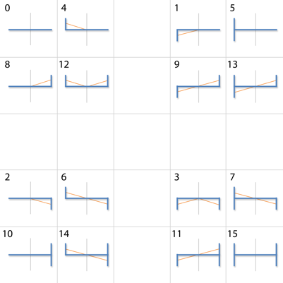
观察此图和对应分支代码,可以发现area函数的坐标系原点是在left处,即最左边edge那里。以这里为原点,+x方向朝右,+y方向朝下。
# Calculates the area under the line p1->p2, for the pixel x..x+1:
def area(p1, p2, x):
    d = p2[0] - p1[0], p2[1] - p1[1]
    x1 = float(x)
    x2 = x + 1.0
    y1 = p1[1] + d[1] * (x1 - p1[0]) / d[0]
    y2 = p1[1] + d[1] * (x2 - p1[0]) / d[0]
    inside = (x1 >= p1[0] and x1 < p2[0]) or (x2 > p1[0] and x2 <= p2[0]) # 线段[x,x+1]和[p1,p2]需要重叠
    if inside:
        istrapezoid = (copysign(1.0, y1) == copysign(1.0, y2) or
                        abs(y1) < 1e-4 or abs(y2) < 1e-4)
        # 计算是不是梯形(y1和y2同正负号)/直角形(y1或y2的长度为0)
        if istrapezoid:
            a = (y1 + y2) / 2.0 # 梯形面积公式:0.5 * h * (上底+下底) = 0.5 * 1 * (y1 + y2)
            if a < 0.0: # y1和y2都在top edge线下方
                return abs(a), 0.0
            else:
                return 0.0, abs(a)
        else: # [p1,p2]和top edge交叉了,形成2个三角形
            x = -p1[1] * d[0] / d[1] + p1[0]
            a1 = y1 *        modf(x)[0]  / 2.0 if x > p1[0] else 0.0
            a2 = y2 * (1.0 - modf(x)[0]) / 2.0 if x < p2[0] else 0.0
            a = a1 if abs(a1) > abs(a2) else -a2
            if a < 0.0:
                return abs(a1), abs(a2)
            else:
                return abs(a2), abs(a1)
    else:
        return 0.0, 0.0
函数说明写着area函数算的是p1到p2这条线段下,x到x+1范围内的面积,x参数其实就是等于left,因为16个pattern都是传入了left。所以[x, x+1]就是[left,left+1],又因为坐标系原点在最左边,[left,left+1]指的其实就是当前像素的左边界和右边界(一个像素的宽度为1)。所以area的任务就是要算出p1-p2把当前像素切开了多大面积。
再就是斜向的情况:
如果能完全理解ortho的情况,diag的就触类旁通了。这里暂时跳过。(这套SMAA太多细节了,每个点都搞懂实在不容易)
search算法
(待续)
用weightTex混合原图像(Pass 3)
总结
SMAA的优点:
- 强配置性,可以根据需要决定使用SMAA 1x/SMAA t2x/SMAA 4x
- SMAA 4x的性能和质量足以抗衡SSAA,低配的SMAA 1x对低端机也足够用了
- 支持defer框架
SMAA的缺点:
- 流程太复杂,代码各种trick,仅读论文是看不懂代码的。只能边看代码边读论文,结合地去理解。
- 需要预生成areaTex、searchTex,维护shader之外还得维护2个py脚本,定制修改SMAA比较复杂。
我说的缺点可能比较naive,说不定对大佬来说这套SMAA并不复杂。
本文仅介绍SMAA 1x的技术原理,至于SMAA t2x和SMAA 4x需要用到temporal reprojection和supersampliing,就是更进一步的话题了。
最终效果
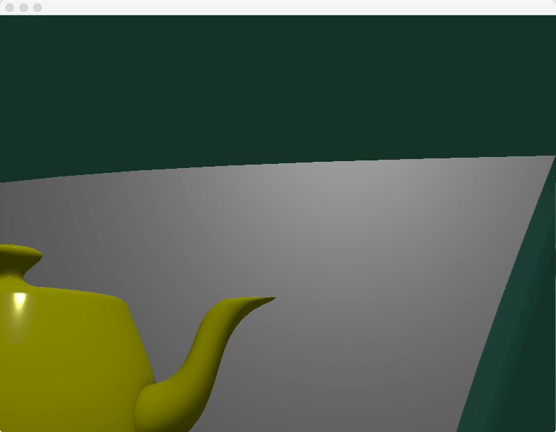
原始图像:
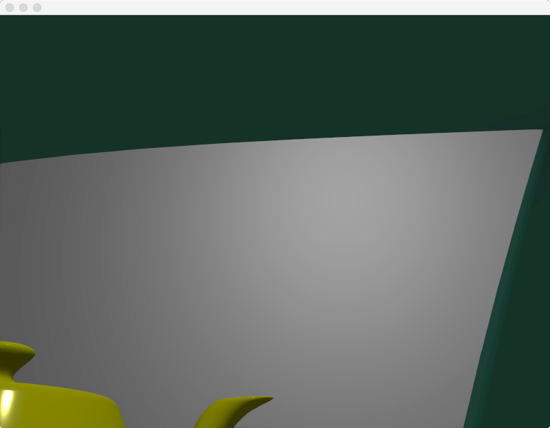
经过SMAA 1x过滤后:
资料
写作不易,您的支持是我写作的动力!